
Multicollinearity is a frequent challenge in econometric analysis, especially in models involving multiple explanatory variables. It occurs when two or more independent variables in a regression model are highly correlated, making it difficult to determine their individual effects on the dependent variable. This correlation between predictors can lead to unreliable coefficient estimates, ultimately compromising the validity of the econometric model. In this post, we will delve into:
- The definition and effects of multicollinearity
- Methods to detect multicollinearity in your models
- Approaches to solving multicollinearity for accurate results
- A practical example using economic data
Defining Multicollinearity
In multiple regression models, a key assumption is that the independent variables are not perfectly correlated with one another. However, multicollinearity arises when this assumption is violated—when two or more independent variables are strongly correlated. This interdependence can distort the estimation process, making it challenging to isolate the individual effects of each explanatory variable on the dependent variable.
Multicollinearity can be categorized into two types:
- Perfect Multicollinearity
This occurs when an explanatory variable is an exact linear function of another. For instance, if ( X_2 = 5 + 2.5 X_1 ), there is a perfect linear relationship between ( X_1 ) and ( X_2 ). Such scenarios render the regression model unsolvable, as it becomes impossible to distinguish the unique contributions of each variable.
- Imperfect (or Near) Multicollinearity
This is more common and occurs when the relationship between two or more independent variables is strong but not exact. It often arises due to a small error term or minor variations in the relationship between the variables.
Example of Multicollinearity
To better understand the concept, imagine a regression model estimating the impact of income and liquid assets on household consumption. Since income and liquid assets are closely related—higher-income households typically have more assets—it becomes difficult to determine which variable is driving changes in consumption. This overlap between income and liquid assets introduces multicollinearity into the model, resulting in inflated standard errors and unstable coefficient estimates.
Effects of Multicollinearity on Econometric Models
Multicollinearity effects regression models in various ways, influencing both the reliability of the estimates and the conclusions drawn from them:
Inflated Standard Errors
Multicollinearity increases the variance of the estimated coefficients, leading to larger standard errors. This makes it difficult to determine which variables are statistically significant, as even theoretically important predictors may appear insignificant.
Unreliable t-tests
When standard errors are inflated, it undermines the reliability of t-tests. As a result, variables that should be statistically significant might appear otherwise, affecting the interpretation of results.
Unstable Coefficients
With multicollinearity, coefficients can change dramatically with the inclusion or exclusion of other variables. This instability means that even small changes in the dataset can produce large changes in the estimated parameters, leading to inconsistent conclusions.
Misleading Model Inference
Multicollinearity can lead to incorrect interpretations about the relationship between variables, as the model becomes more sensitive to minor data changes. This can undermine the overall reliability of the regression analysis.
In econometric analysis, detecting and addressing multicollinearity is crucial to ensure that the model’s estimates are meaningful and robust.
Detecting Multicollinearity
Several methods can be used to detect multicollinearity, ranging from basic visual tools to advanced statistical tests:
Pairwise Correlation Coefficients
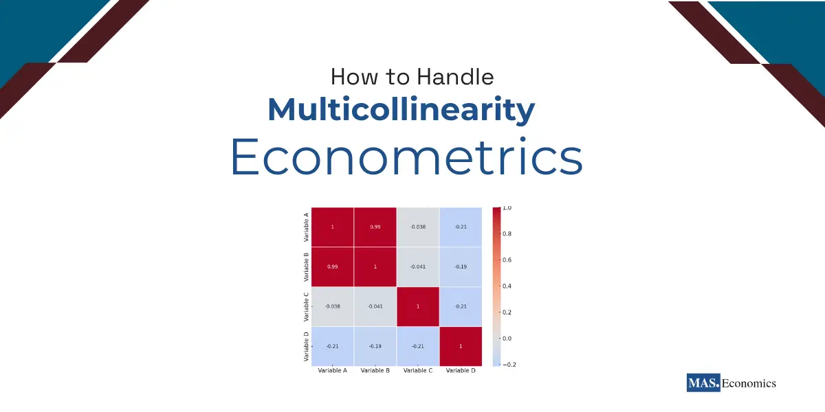
A straightforward method for detecting multicollinearity is to examine the pairwise correlation between explanatory variables. High correlation coefficients (close to +1 or -1) indicate a strong linear relationship, suggesting potential multicollinearity. This method works best in models with a few predictors.
Table 1: Correlation Matrix Showing High Correlations, visualized using a heatmap. The matrix displays the pairwise correlation coefficients between explanatory variables. As seen in the matrix, there is a high positive correlation between Variable A and Variable B (0.99), suggesting potential multicollinearity between these variables. Lower correlations are observed between other variable pairs, indicating weaker relationships. This matrix is useful for detecting multicollinearity in regression models.
Variance Inflation Factor (VIF)
The Variance Inflation Factor (VIF) is a widely used measure for assessing the degree of multicollinearity in a regression model. It quantifies how much the variance of a regression coefficient is inflated due to multicollinearity. The formula for VIF is:
[
VIF_i = frac{1}{1 – R_i^2}
]
- ( R_i^2 ) is the ( R^2 ) value obtained from regressing the ( i )-th explanatory variable on all other predictors in the model.
A VIF greater than 10 is commonly considered a sign of high multicollinearity, though, in some fields, thresholds may vary.
Eigenvalue Method
The eigenvalue method involves calculating the eigenvalues of the correlation matrix of the explanatory variables. Small eigenvalues indicate potential multicollinearity. The condition number, calculated as the ratio of the largest to the smallest eigenvalue, is another indicator—values exceeding 30 often suggest severe multicollinearity.
Solving Multicollinearity
Once multicollinearity is detected, several strategies can be applied to mitigate its impact:
Removing One of the Collinear Variables
When two variables are highly correlated, removing one of them can reduce multicollinearity. This method is most effective when the removed variable does not contribute significantly to the model’s explanatory power.
Combining Variables
If variables measure similar economic phenomena, they can be combined into a single index. For example, rather than including both income and liquid assets separately, one could use a composite measure of wealth. This approach helps to reduce redundancy in the model.
Principal Component Analysis (PCA)
Principal Component Analysis (PCA) is a statistical method that transforms a set of correlated variables into a smaller set of uncorrelated components. By using these components as explanatory variables, PCA effectively reduces the dimensionality of the model and eliminates multicollinearity.
Ridge Regression
Ridge Regression is a regularization technique that helps to stabilize regression coefficients when multicollinearity is present. It introduces a penalty parameter ( lambda ), which shrinks the coefficients towards zero, reducing their variance and mitigating multicollinearity:
[
hat{beta}_{ridge} = (X’X + lambda I)^{-1} X’Y
]
- ( lambda ) is the regularization parameter.
Ridge regression is especially useful in high-dimensional data where traditional methods might struggle.
Practical Example of Multicollinearity in Economic Data
Consider an example analyzing the impact of GDP growth, inflation, and unemployment on consumer spending. Given the inverse relationship between inflation and unemployment (as described by the Phillips curve), multicollinearity is likely.
Detecting Multicollinearity
Calculating the correlation matrix reveals that inflation and unemployment correlate 0.85, suggesting multicollinearity. We also compute the VIF values and find that both variables have VIF values above 10, further confirming the issue.
Solving Multicollinearity
To address this, we use Principal Component Analysis (PCA) to create a new variable that captures the combined effect of inflation and unemployment on consumer spending. This new variable reduces multicollinearity and stabilizes the regression coefficients, leading to a more reliable model.
Conclusion
Multicollinearity is a frequent challenge in econometric analysis, particularly in models with multiple explanatory variables. It can obscure the true relationship between variables, leading to unreliable estimates and unstable models. However, with proper detection techniques like VIF and correlation matrices, and solutions such as PCA, ridge regression, or simplifying the model, econometricians can mitigate its adverse effects. Addressing multicollinearity is critical for ensuring the accuracy and interpretability of econometric models, enabling more robust conclusions and data-driven decisions.
In the next post, we will how to select the best econometric model for your data.
Thanks for reading! If you found this helpful, share it with friends and spread the knowledge.
Happy learning with MASEconomics


